CRC算法原理与实现05——并行计算公式推导

浏览量 174

CRC算法原理与实现系列文章：

CRC算法原理与实现01——概述 – 徐晓康的博客

CRC算法原理与实现02——数学原理与模2运算 – 徐晓康的博客

CRC算法原理与实现03——参数说明、计算步骤与应用场景 – 徐晓康的博客

CRC算法原理与实现04——软硬件实现方法简介 – 徐晓康的博客

CRC算法原理与实现05——并行计算公式推导 – 徐晓康的博客

CRC算法原理与实现06——自编Python计算任意CRC – 徐晓康的博客

CRC算法原理与实现07——Verilog单步计算任意CRC – 徐晓康的博客

CRC算法原理与实现08——Verilog多步计算任意CRC – 徐晓康的博客

CRC算法原理与实现09——C语言计算任意CRC – 徐晓康的博客

前言

本文是CRC并行计算的理论基础。为了理解CRC并行计算的原理，我看了很多论文，这套方法在一些论文中应该已经讲过了，但遗憾的是，很少有文章能把它讲清楚。本文从最基础的数学原理出发，力求详细且不跳步，有点线性代数基础的同学应该能顺利理解。

并行算法是从基础的移位寄存器法中总结出来的，下面详细推导出并行计算的公式。

一. CRC并行计算公式推导

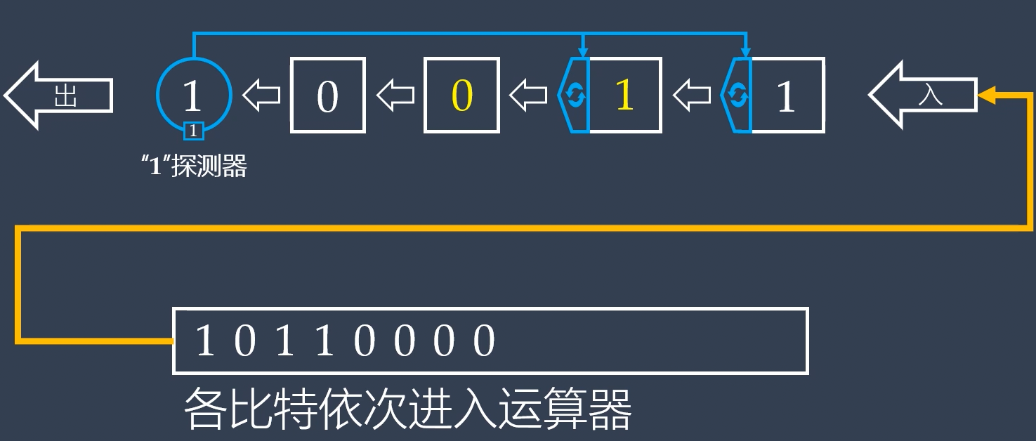
以串行左移反馈移位寄存器为参考，考虑用数学公式按左移反馈的步骤，一步步推导出并行计算的公式。

设宽度为n的CRC寄存器的初始值为C，用行向量表示，有：

$\displaylines{ C=\left[ \begin{array}{l} c_{n-1}& c_{n-2}& \cdots& c_0\\ \end{array} \right] } \\$

生成多项式用G表示，有：

$\displaylines{ G=\left[ g_{n-1}\,\,g_{n-2}\,\,\cdots \,\,g_0 \right] } \\$

设输入数据的位宽为k，用行向量D表示，有：

$\displaylines{ D=\left[ \begin{array}{l} d_{k-1}& d_{k-2}& \cdots& d_0\\ \end{array} \right] } \\$

设CRC寄存器左移移位并反馈后的状态为 $C^{\prime}$ ，有：

$\displaylines{ C^{\prime}=\left[ \begin{array}{l} {c_{n-1}}^{\prime}& {c_{n-2}}^{\prime}& \cdots& {c_0}^{\prime}\\ \end{array} \right] } \\$

根据左移反馈的运算机制，当原寄存器的最高位为1时，CRC左移一位，并于生成多项式G进行异或；当原寄存器最高位为0时，CRC左移一位，不异或，由此可得到如下递推关系：

$\displaylines{ {c_{n-1}}^{\prime}=\left( c_{n-1}\cdot g_{n-1} \right) \oplus c_{n-2} \\ {c_{n-2}}^{\prime}=\left( c_{n-1}\cdot g_{n-2} \right) \oplus c_{n-3} \\ \vdots \\ {c_1}^{\prime}=\left( c_{n-1}\cdot g_1 \right) \oplus c_0 \\ {c_0}^{\prime}=\left( c_{n-1}\cdot g_0 \right) \oplus d_{k-1} \\ \text{其中，}\oplus \text{表示异或运算} } \\$

这里的所有符号变量的值都是二进制的，不是0就是1，注意 $c_{n-1}$ 为原寄存器的最高位的值。

两个数的异或运算，等价于两个数加法后模2，所以上式可改写为：

$\displaylines{ {c_{n-1}}^{\prime}=\left( c_{n-1}\cdot g_{n-1}+c_{n-2} \right) \,\,mod2 \\ {c_{n-2}}^{\prime}=\left( c_{n-1}\cdot g_{n-2}+c_{n-3} \right) mod2 \\ \vdots \\ {c_1}^{\prime}=\left( c_{n-1}\cdot g_1+c_0 \right) mod2 \\ {c_0}^{\prime}=\left( c_{n-1}\cdot g_0+d_{k-1} \right) mod2 \\ \text{其中，}mod2\text{为模}2\text{运算} } \\$

根据上述表达式，可以构建 $C^{\prime}$ 与C之间的状态转移矩阵表达式，称为单步状态转移公式，有：

$\displaylines{ C^{\prime}=\left( C\cdot T+D_1 \right) mod2 } \\$

其中，T为状态转移矩阵，它第一行为生成多项式G的系数，左下为n-1×n-1的单位矩阵，右下全0，有：

$\displaylines{ T=\left[ \begin{matrix} g_{n-1}& g_{n-2}& \cdots& g_1& g_0\\ 1& 0& \cdots& 0& 0\\ 0& 1& \cdots& 0& 0\\ \vdots& \vdots& \ddots& \vdots& \vdots\\ 0& 0& \cdots& 1& 0\\ \end{matrix} \right] } \\$

$D_1$ 为输入向量的扩展形式，为n个元素的行向量，最后一个元素为 $d_{k-1}$ ，即输入数据的最高位，其余位全0，有：

$\displaylines{ D_1=\left[ \begin{array}{l} 0& 0& \cdots& 0& d_{k-1}\\ \end{array} \right] } \\$

我们来验证一下这个表达式是否正确，有：

$\displaylines{ \left( C\cdot T+D_1 \right) mod2= \\ \left( \begin{array}{c} \left[ \begin{array}{l} c_{n-1}& c_{n-2}& \cdots& c_0\\ \end{array} \right] \cdot \left[ \begin{matrix} g_{n-1}& g_{n-2}& \cdots& g_1& g_0\\ 1& 0& \cdots& 0& 0\\ 0& 1& \cdots& 0& 0\\ \vdots& \vdots& \ddots& \vdots& \vdots\\ 0& 0& \cdots& 1& 0\\ \end{matrix} \right]\\ +\left[ \begin{array}{l} 0& 0& \cdots& 0& d_{k-1}\\ \end{array} \right]\\ \end{array} \right) mod2 } \\$

根据矩阵乘法运算的规则，有：

$\displaylines{ \text{第}n-1\text{个元素：}\left( c_{n-1}\cdot g_{n-1}+c_{n-2} \right) mod2={c_{n-1}}^{\prime} \\ \text{第}n-2\text{元素：}\left( c_{n-1}\cdot g_{n-2}+c_{n-3} \right) mod2={c_{n-2}}^{\prime} \\ \vdots \\ \text{第}1\text{个元素：}\left( c_{n-1}\cdot g_1+c_0 \right) mod2={c_1}^{\prime} \\ \text{第}0\text{个元素：}\left( c_{n-1}\cdot g_0+d_{k-1} \right) mod2={c_0}^{\prime} } \\$

所以，这里证明了单步状态转移公式的正确性。

根据这个公式进一步推导，我们就能得到多步状态转移公式，也就是并行计算公式了。

现在，考虑 $C^{\prime}$ 下一步的状态 $C^{''}$ ，根据单步状态转移公式，有：

$\displaylines{ C^{''}=\left( C^{\prime}\cdot T+D_2 \right) mod2 } \\$

其中， $D_2=\left[ \begin{array}{l} 0& 0& \cdots& d_{k-2}\\ \end{array} \right]$ ，它表示原始数据的次高位现在移入寄存器了。

把 $C^{\prime}$ 展开，有：

$\displaylines{ C^{''}=\left( C^{\prime}\cdot T+D_2 \right) mod2 \\ =\left( \left( \left( C\cdot T+D_1 \right) mod2 \right) \cdot T+D_2 \right) mod2 } \\$

这个表达式就有点复杂了，考虑mod2运算的性质：

$\displaylines{ \left( A\cdot B \right) mod2=\left( Amod2 \right) \cdot \left( Bmod2 \right) } \\$

矩阵A与B的乘积模2等于A模2乘以B模2。另一个性质：

$\displaylines{ \left( A+B \right) mod2=\left( \left( Amod2 \right) +\left( Bmod2 \right) \right) mod2 } \\$

矩阵A与B的和模2等于A模2和B模2的和再模2。

因为T和 $D_2$ 每个元素为0或1，所以，

$\displaylines{ T=Tmod2 \\ D_2=D_2mod2 } \\$

所以， $C^{''}$ 可以写为：

$\displaylines{ C^{''}=\left( \left( \left( C\cdot T+D_1 \right) mod2 \right) \cdot Tmod2+D_2 \right) mod2 \\ =\left( \left( \left( C\cdot T+D_1 \right) \cdot T \right) mod2+D_2 \right) mod2 \\ =\left( \left( C\cdot T\cdot T+D_1\cdot T \right) mod2+D_2mod2 \right) mod2 \\ =\left( C\cdot T\cdot T+D_1\cdot T+D_2 \right) mod2 \\ =\left( C\cdot T^2+D_1\cdot T+D_2 \right) mod2 } \\$

下面计算一下， $D_1\cdot T$ ，有：

$\displaylines{ D_1\cdot T=\left[ \begin{array}{l} 0& 0& \cdots& d_{k-1}\\ \end{array} \right] \cdot \left[ \begin{matrix} g_{n-1}& g_{n-2}& \cdots& g_1& g_0\\ 1& 0& \cdots& 0& 0\\ 0& 1& \cdots& 0& 0\\ \vdots& \vdots& \ddots& \vdots& \vdots\\ 0& 0& \cdots& 1& 0\\ \end{matrix} \right] \\ =\left[ \begin{array}{l} 0& 0& \cdots& d_{k-1}& 0\\ \end{array} \right] } \\$

所以，可以认为 $D_1\cdot T$ 对 $D_1$ 的作用是：使 $D_1$ 左移一位，低位补0。

考虑 $D_1\cdot T+D_2$ ，有：

$\displaylines{ D_1\cdot T+D_2 \\ =\left[ \begin{array}{l} 0& 0& \cdots& d_{k-1}& 0\\ \end{array} \right] +\left[ \begin{array}{l} 0& 0& \cdots& 0& d_{k-2}\\ \end{array} \right] \\ =\left[ \begin{array}{l} 0& 0& \cdots& d_{k-1}& d_{k-2}\\ \end{array} \right] } \\$

令 $D^{\prime}=D_1$ ，

令 $D^{''}=\left[ \begin{array}{l} 0& 0& \cdots& d_{k-1}& d_{k-2}\\ \end{array} \right]$ ，这里 $D^{''}$ 可以理解为原始数据D左移进入一个初始值全0的寄存器，左移了两位，有：

$\displaylines{ C^{\prime}=\left( C\cdot T+D^{\prime} \right) mod2 \\ C^{''}=\left( C\cdot T^2+D^{''} \right) mod2 } \\$

那么 $C^{''}$ 的下一个状态 $C^{'''}$ 呢，容易推导出：

$\displaylines{ C^{'''}=\left( C\cdot T^3+D^{'''} \right) mod2 } \\$

其中， $D^{'''}=\left[ \begin{array}{l} 0& \cdots& d_{k-1}& d_{k-2}& d_{k-3}\\ \end{array} \right]$ 。

到这里规律就显而易见了，因为’，” 和 ”’表示的步骤有限，令：

$\displaylines{ \text{初始状态：}C\left( 0 \right) =C\text{，}D\left( 0 \right) =\left[ \begin{array}{l} 0& 0& \cdots& 0\\ \end{array} \right] \\ \text{下个状态：}C\left( 1 \right) =C^{\prime}\text{，}D\left( 1 \right) =D^{\prime} \\ \text{再下个状态：}C\left( 2 \right) =C^{''}\text{，}D\left( 2 \right) =D^{''} \\ \text{依次类推} } \\$

状态转换公式可写为：

$\displaylines{ C\left( 1 \right) =\left( C\left( 0 \right) \cdot T+D\left( 1 \right) \right) mod2 \\ C\left( 2 \right) =\left( C\left( 1 \right) \cdot T^2+D\left( 2 \right) \right) mod2 \\ \vdots \\ C\left( i \right) =\left( C\left( 0 \right) \cdot T^i+D\left( i \right) \right) mod2\text{，其中，}0\leqslant i\leqslant n \\ \vdots \\ C\left( n \right) =\left( C\left( 0 \right) \cdot T^n+D\left( n \right) \right) mod2 } \\$

注意：

$C\left( 0 \right)$ 为CRC寄存器的初始值，对于从最初开始计算CRC来说，它总是0。只有分多步计算CRC时，前面已经算过至少一次了，C(0)作为后续步骤的CRC寄存器初始值。
这里隐含了数学上对矩阵零次方的定义，即一个n×n的矩阵的零次方 = 单位矩阵，即对角线元素为1，其余位全0的矩阵。

从上述公式我们可以看出，i为移位的步数，状态转移矩阵T由生成多项式决定，D(n)由输入数据和计算步数决定，所以，这里就得到了移位寄存器移动i位后的状态与生成多项式和输入数据的关系。

此公式是并行CRC计算的理论基础。

二. CRC并行计算公式验证

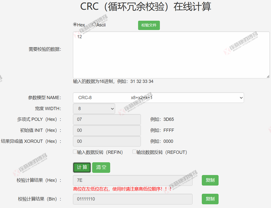
2.1 CRC-8

多项式：0x07（0000_0111）
初始异或值：0x00
输入反转：无
输出反转：无
最终异或值：0x00

输入数据为0x12，注意在进行CRC计算时，输入数据需要先补0再异或，所以实际参与运算的输入数据为0x1200，有：

$\displaylines{ T=\left[ \begin{array}{l} 0& 0& 0& 0& 0& 1& 1& 1\\ 1& 0& 0& 0& 0& 0& 0& 0\\ 0& 1& 0& 0& 0& 0& 0& 0\\ 0& 0& 1& 0& 0& 0& 0& 0\\ 0& 0& 0& 1& 0& 0& 0& 0\\ 0& 0& 0& 0& 1& 0& 0& 0\\ 0& 0& 0& 0& 0& 1& 0& 0\\ 0& 0& 0& 0& 0& 0& 1& 0\\ \end{array} \right] } \\$

CRC寄存器初始值为0，有：

$\displaylines{ C\left( 8 \right) =C\left( 0 \right) \cdot T^8+D\left( 8 \right) =D\left( 8 \right) } \\$

以C(8)为初始值，有最终的CRC寄存器值：

$\displaylines{ C\left( 16 \right) =C\left( 8 \right) \cdot T^8+D\left( 9:16 \right) } \\$

其中， $D\left( 9:16 \right)$ 为输入数据的第9~16位，实际是补的0。有：

$\displaylines{ C\left( 16 \right) =\left( D\left( 8 \right) \cdot T^8 \right) mod2 \\ =\left( \left[ \begin{array}{l} 0& 0& 0& 1& 0& 0& 1& 0\\ \end{array} \right] \cdot \left[ \begin{array}{l} 0& 0& 0& 0& 0& 1& 1& 1\\ 1& 0& 0& 0& 0& 0& 0& 0\\ 0& 1& 0& 0& 0& 0& 0& 0\\ 0& 0& 1& 0& 0& 0& 0& 0\\ 0& 0& 0& 1& 0& 0& 0& 0\\ 0& 0& 0& 0& 1& 0& 0& 0\\ 0& 0& 0& 0& 0& 1& 0& 0\\ 0& 0& 0& 0& 0& 0& 1& 0\\ \end{array} \right] ^8 \right) mod2 } \\$

这个我们写个Python程序算一下：

import numpy as np

# 定义矩阵 D(8)
D = np.array([[0, 0, 0, 1, 0, 0, 1, 0]])

# 定义矩阵 T
T = np.array([
    [0, 0, 0, 0, 0, 1, 1, 1],
    [1, 0, 0, 0, 0, 0, 0, 0],
    [0, 1, 0, 0, 0, 0, 0, 0],
    [0, 0, 1, 0, 0, 0, 0, 0],
    [0, 0, 0, 1, 0, 0, 0, 0],
    [0, 0, 0, 0, 1, 0, 0, 0],
    [0, 0, 0, 0, 0, 1, 0, 0],
    [0, 0, 0, 0, 0, 0, 1, 0]
])

# 计算 T^8
T_power_8 = np.linalg.matrix_power(T, 8)

# 计算 C(16) = D(8) * T^8
C = np.dot(D, T_power_8) % 2

# 输出结果
print("T^8:")
print(T_power_8)
print("\nC(16):")
print(C)

运行结果：

T^8:
[[1 0 0 0 1 2 2 1]
 [1 1 0 0 0 1 1 1]
 [1 1 1 0 0 0 0 0]
 [0 1 1 1 0 0 0 0]
 [0 0 1 1 1 0 0 0]
 [0 0 0 1 1 1 0 0]
 [0 0 0 0 1 1 1 0]
 [0 0 0 0 0 1 1 1]]

C(16):
[[0 1 1 1 1 1 1 0]]

对照CRC计算网站上计算的结果：两者一致。

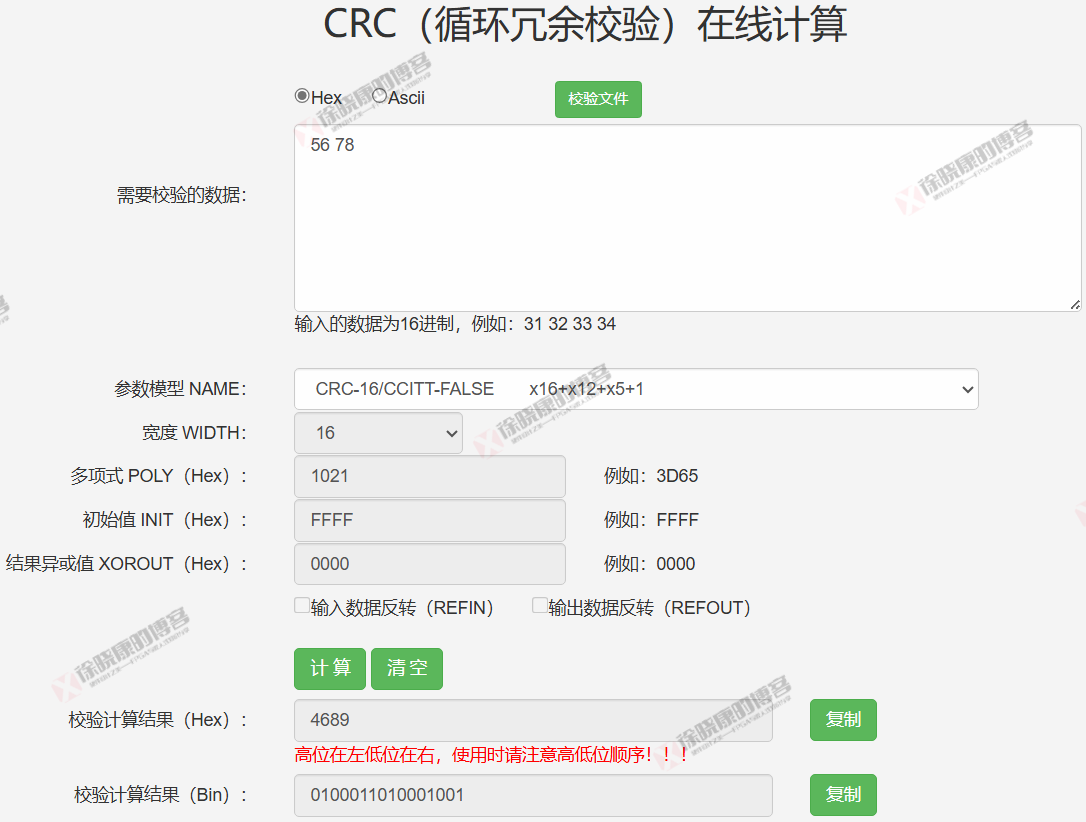
2.2 CRC-16-CCITT-FALSE

多项式：0x1021（0001_0000_0010_0001）
初始异或值：0xFFFF
输入反转：无
输出反转：无
最终异或值：0x0000

输入数据0x5678，先补0变为0x56780000，再与初始异或值异或，为0xA9870000，推导一下输出表达式：

$\displaylines{ C\left( 16 \right) =\left( C\left( 0 \right) \cdot T^{16}+D\left( 16 \right) \right) mod2 \\ C\left( 32 \right) =\left( C\left( 16 \right) \cdot T^{16}+D\left( 17:32 \right) \right) mod2 \\ =\left( C\left( 0 \right) \cdot T^{32}+D\left( 16 \right) \cdot T^{16}+D\left( 17:32 \right) \right) mod2 \\ =\left( D\left( 16 \right) \cdot T^{16} \right) mod2 } \\$

对应Python程序：

import numpy as np

# 定义矩阵 D(16) 0xA987
D16 = np.array([[1, 0, 1, 0, 1, 0, 0, 1, 1, 0, 0, 0, 0, 1, 1, 1]])

# 定义矩阵 T, G=0x1021
T = np.array([
    [0, 0, 0, 1, 0, 0, 0, 0, 0, 0, 1, 0, 0, 0, 0, 1],
    [1, 0, 0, 0, 0, 0, 0, 0, 0, 0, 0, 0, 0, 0, 0, 0],
    [0, 1, 0, 0, 0, 0, 0, 0, 0, 0, 0, 0, 0, 0, 0, 0],
    [0, 0, 1, 0, 0, 0, 0, 0, 0, 0, 0, 0, 0, 0, 0, 0],
    [0, 0, 0, 1, 0, 0, 0, 0, 0, 0, 0, 0, 0, 0, 0, 0],
    [0, 0, 0, 0, 1, 0, 0, 0, 0, 0, 0, 0, 0, 0, 0, 0],
    [0, 0, 0, 0, 0, 1, 0, 0, 0, 0, 0, 0, 0, 0, 0, 0],
    [0, 0, 0, 0, 0, 0, 1, 0, 0, 0, 0, 0, 0, 0, 0, 0],
    [0, 0, 0, 0, 0, 0, 0, 1, 0, 0, 0, 0, 0, 0, 0, 0],
    [0, 0, 0, 0, 0, 0, 0, 0, 1, 0, 0, 0, 0, 0, 0, 0],
    [0, 0, 0, 0, 0, 0, 0, 0, 0, 1, 0, 0, 0, 0, 0, 0],
    [0, 0, 0, 0, 0, 0, 0, 0, 0, 0, 1, 0, 0, 0, 0, 0],
    [0, 0, 0, 0, 0, 0, 0, 0, 0, 0, 0, 1, 0, 0, 0, 0],
    [0, 0, 0, 0, 0, 0, 0, 0, 0, 0, 0, 0, 1, 0, 0, 0],
    [0, 0, 0, 0, 0, 0, 0, 0, 0, 0, 0, 0, 0, 1, 0, 0],
    [0, 0, 0, 0, 0, 0, 0, 0, 0, 0, 0, 0, 0, 0, 1, 0]
])

# 计算 T^16
T_power_16 = np.linalg.matrix_power(T, 16)

# 计算 C(32) = D(16) * T^16
C = np.dot(D16, T_power_16)
C = C % 2

# 输出结果
print("T^16:")
print(T_power_16)
print("\nC(32):")
print(C)

运行结果：

T^16:
[[2 0 0 3 1 0 1 1 1 0 2 1 1 0 0 2]
 [2 2 0 0 1 1 0 1 1 1 0 0 1 1 0 0]
 [0 2 2 0 0 1 1 0 1 1 1 0 0 1 1 0]
 [0 0 2 2 0 0 1 1 0 1 1 1 0 0 1 1]
 [1 0 0 2 1 0 0 1 1 0 1 0 1 0 0 1]
 [1 1 0 0 1 1 0 0 1 1 0 0 0 1 0 0]
 [0 1 1 0 0 1 1 0 0 1 1 0 0 0 1 0]
 [0 0 1 1 0 0 1 1 0 0 1 1 0 0 0 1]
 [1 0 0 1 0 0 0 1 1 0 0 0 1 0 0 0]
 [0 1 0 0 1 0 0 0 1 1 0 0 0 1 0 0]
 [0 0 1 0 0 1 0 0 0 1 1 0 0 0 1 0]
 [0 0 0 1 0 0 1 0 0 0 1 1 0 0 0 1]
 [1 0 0 0 0 0 0 1 0 0 0 0 1 0 0 0]
 [0 1 0 0 0 0 0 0 1 0 0 0 0 1 0 0]
 [0 0 1 0 0 0 0 0 0 1 0 0 0 0 1 0]
 [0 0 0 1 0 0 0 0 0 0 1 0 0 0 0 1]]

C(32):
[[0 1 0 0 0 1 1 0 1 0 0 0 1 0 0 1]]

对照CRC计算网站上计算的结果：两者一致。

三. 通用CRC并行计算公式推导

回顾一下上文推导的CRC并行公式：

$\displaylines{ C\left( i \right) =\left( C\left( 0 \right) \cdot T^i+D\left( i \right) \right) mod2\text{，其中，}0\leqslant i\leqslant n } \\$

此公式一次可以并行计算i位，i最大为CRC的宽度n，意思是最多一次算n位。但输入数据在补0后，位宽总是比CRC宽度要大，有没有公式可以一次性算完所有位呢？当然可以，只需要基于这个公式再推导一下：

设CRC位宽为N，用大写N替代小写n，表示对于一个确定的CRC，位宽总是固定的，有：

$\displaylines{ C\left( N \right) =\left( C\left( 0 \right) \cdot T^N+D\left( N \right) \right) mod2 } \\$

将 $C\left( N \right)$ 视为一下步计算的CRC寄存器初始状态，有：

$\displaylines{ C\left( N+i \right) =\left( C\left( N \right) \cdot T^i+D\left( N+1:N+i \right) \right) mod2 \\ =\left( \left( C\left( 0 \right) \cdot T^N+D\left( N \right) \right) \cdot T^i+D\left( N+1:N+i \right) \right) mod2 \\ =\left( C\left( 0 \right) \cdot T^{N+i}+D\left( N \right) \cdot T^i+D\left( N+1:N+i \right) \right) mod2 \\ \text{其中，}0\leqslant i\leqslant N } \\$

由此式可以推导出， $C\left( 2N \right)$ 的表达式：

$\displaylines{ C\left( 2N \right) =\left( C\left( 0 \right) \cdot T^{2N}+D\left( N \right) \cdot T^N+D\left( N+1:2N \right) \right) mod2 } \\$

那么超过2N个bit呢？有：

$\displaylines{ C\left( 2N+i \right) =\left( C\left( 2N \right) \cdot T^i+D\left( 2N+1:2N+i \right) \right) mod2 \\ =\left( \begin{array}{c} \left( C\left( 0 \right) \cdot T^{2N}+D\left( N \right) \cdot T^N+D\left( N+1:2N \right) \right) \cdot T^i\\ +D\left( 2N+1:2N+i \right)\\ \end{array} \right) mod2 \\ =\left( \begin{array}{c} C\left( 0 \right) \cdot T^{2N+i}+D\left( N \right) \cdot T^{N+i}+D\left( N+1:2N \right) \cdot T^i\\ +D\left( 2N+1:2N+i \right)\\ \end{array} \right) mod2 \\ \text{其中，}0\leqslant i\leqslant N } \\$

由此可以总结出规律：

$\displaylines{ C\left( N\cdot j+i \right) =\left( \begin{array}{c} C\left( 0 \right) \cdot T^{N\cdot j+i}\\ +D\left( N \right) \cdot T^{N\cdot \left( j-1 \right) +i}\\ +D\left( N+1:2N \right) \cdot T^{N\cdot \left( j-2 \right) +i}\\ +\cdots\\ +D\left( N\cdot \left( j-1 \right) +1:N\cdot j \right) \cdot T^i\\ +D\left( N\cdot j+1:N\cdot j+i \right)\\ \end{array} \right) mod2 \\ \text{其中，}0\leqslant i\leqslant N\text{，}j\geqslant 0 } \\$

这就是通用的CRC并行计算公式，它实现了任意位宽数据的并行计算。

四. 通用CRC并行计算公式验证

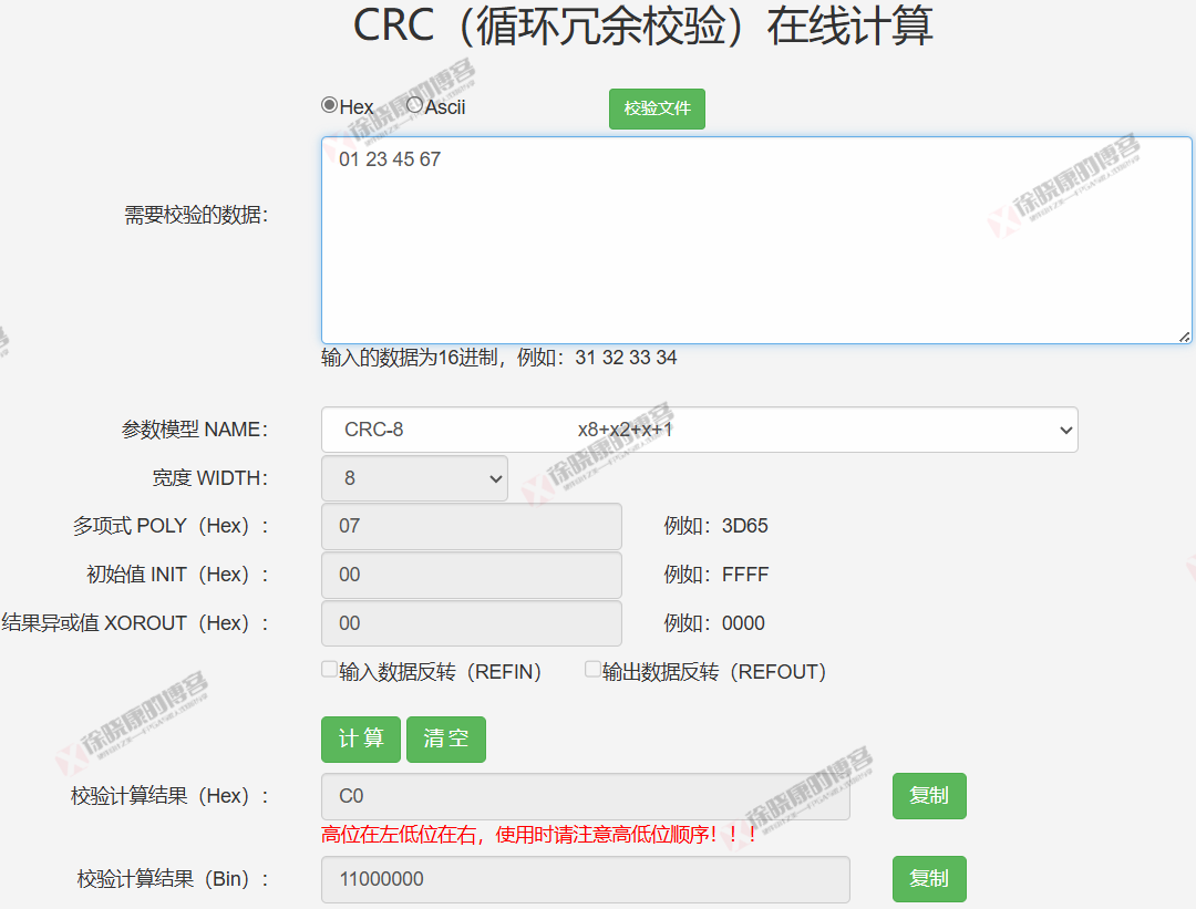
4.1 CRC-8

输入数据为0x1234567，补0后为0x123456700，一次算完：

$\displaylines{ N=8,j=4,i=4 \\ C\left( N\cdot 4+4 \right) =\left( \begin{array}{c} C\left( 0 \right) \cdot T^{N\cdot 4+4}\\ +D\left( N \right) \cdot T^{N\cdot 3+4}\\ +D\left( N+1:2N \right) \cdot T^{N\cdot 2+4}\\ +D\left( 2N+1:3N \right) \cdot T^{N+4}\\ +D\left( 3N+1:4N \right) \cdot T^4\\ +D\left( 4N+1:4N+4 \right)\\ \end{array} \right) mod2 \\ =0+0x12\cdot T^{28}+0x34\cdot T^{20}+0x56\cdot T^{12}+0x70\cdot T^4+0 } \\$

编写Python代码：

import numpy as np

# 定义矩阵 D(8) D(9:16) D(17:24) D(25:32)
D8 = np.array([[0, 0, 0, 1, 0, 0, 1, 0]]) # 0x12
D9_16 = np.array([[0, 0, 1, 1, 0, 1, 0, 0]]) # 0x34
D17_24 = np.array([[0, 1, 0, 1, 0, 1, 1, 0]]) # 0x56
D25_32 = np.array([[0, 1, 1, 1, 0, 0, 0, 0]]) # 0x70


# 定义矩阵 T
T = np.array([
    [0, 0, 0, 0, 0, 1, 1, 1],
    [1, 0, 0, 0, 0, 0, 0, 0],
    [0, 1, 0, 0, 0, 0, 0, 0],
    [0, 0, 1, 0, 0, 0, 0, 0],
    [0, 0, 0, 1, 0, 0, 0, 0],
    [0, 0, 0, 0, 1, 0, 0, 0],
    [0, 0, 0, 0, 0, 1, 0, 0],
    [0, 0, 0, 0, 0, 0, 1, 0]
])

# 计算 T^28 T^20 T^12 T^4
T_power_28 = np.linalg.matrix_power(T, 28)
T_power_20 = np.linalg.matrix_power(T, 20)
T_power_12 = np.linalg.matrix_power(T, 12)
T_power_4 = np.linalg.matrix_power(T, 4)

# 计算 C(36) = D(8)*T^28 + D(9:16)*T^20 + D(17:24)*T^12 + D(25:32)*T^4
C = np.dot(D8, T_power_28) \
    + np.dot(D9_16, T_power_20) \
    + np.dot(D17_24, T_power_12) \
    + np.dot(D25_32, T_power_4)
C = C % 2

# 输出结果
print("\nC(36):")
print(C)

运行结果：

C(36):
[[1 1 0 0 0 0 0 0]]

对照CRC计算网站上计算的结果：两者一致。

4.2 CRC-16-CCITT-FALSE

略，相信各位同学已经理解了公式，自行验证一下吧。

如果本文对你有所帮助，欢迎点赞、转发、收藏、评论让更多人看到，赞赏支持就更好了。

如果对文章内容有疑问，请务必清楚描述问题，留言评论或私信告知我，我看到会回复。

徐晓康的博客持续分享高质量硬件、FPGA与嵌入式知识，软件，工具等内容，欢迎大家关注。